Equations of motion:
1. Forcing of the ocean - general
How do external forces act on the ocean? Gravity creates a pressure gradient that points upward and keeps the water from moving (hydrostatic balance). Others create pressure gradients that cause water to try to flow from high pressure to low pressure. Friction (viscosity) slows the water down. The earth's rotation introduces centrifugal and Coriolis accelerations. (more later).
What equations do physical oceanographers use to describe the ocean?
2. Mass conservation
4. Diffusion:
Occurs because molecules are always in random thermal
motion even if material appears at rest. Diffusion needs a
concentration gradient i.e. more stuff one place than somewhere else.
Described by Fick's Law:
QA = stuff/volume at A = concentrationWe have to measure kappa. If we know it we can answer some questions.
dQ/dx = concentration gradient in direction x
Fick's Law: F = -kappa grad Q, where F is the vector flux.
Flux from A to B = -kappa (QB - QA)/ (B-A) = -kappa dQ/dx
kappa is the diffusion constant:
stuff/cm2/s = kappa stuff/cm3/cm
[ kappa ] = cm2/s (where [ ... ] means "units")
Examples:
(1) In Arctic, surface temperature varies seasonally (T = 86400 x 180 ~
107 sec). Heat diffuses at kappa = 10-3 cm2/s in dirt. How deep (L)
is the seasonal temperature change noticed?
L = sqrt(107 10-3) = 1 m.
(2) How long must year be for seasonal temperature variation to
penetrate 10 m? T = L2/kappa = (107)/10-3 = 109 sec = 30 years!
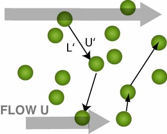
Molecular basis of momentum transport in a gas
Example: Molecules have random thermal speed u' in all directions plus mean flow v in (say) x direction, where v varies with z (height). Molecules go freely a distance L ("mean free path") between collisions. Molecules crossing zo from upper to lower layer carry extra mean momentum v ( z > zo) with it and deposit it in the lower layer after collisions. Thus the upper layer drags the lower layer along.
(figure)
That is to say, tauxz = -rho |u'|L V/??
The quantity |u'|L is the viscosity nu (Greek letter).
In a gas, increasing temperature increases |u'|, so the viscosity goes up.
In a liquid, increasing temperature increases molecular separation, decreases inter-molecular force and the viscosity goes down.
Size of molecular viscosity and diffusivity in sea water:
viscosity: nu = 0.018 cm2/s at 0C; 0.010 at 20C; that is, order (10-2)
diffusivity: kappatemperature = 0.0014 cm2/s
diffusivity: kappasalinity = 0.000013 cm2/sec
Convergence and diffusion: What happens if both advection and diffusion happen at the same time (normal situation)? Advection can sharpen the stuff gradient, while diffusion smooths it. An equilibrium can exist: w = gamma z.
5. Turbulence, Reynolds number, eddy diffusivity (to be covered in a later dynamics lecture )
What is u (velocity) like in the atmosphere/ocean? Is it simple? Consider a flow U in a layer of thickness d, with a viscosity nu. If the ratio Ud/nu is small enough, the flow is laminar - that is, in sliding sheets. Dye in this flow would not disperse.
laminar flow <-> (Uslow)(dwide)/nubigThe quantity Ud/nu = Re is called the Reynolds number. The Reynolds number is a non-dimensional parameter. Re depends on geometry. In the ocean, typical scales are U = 102 cm/sec, d = 4x105 cm, nu = 10-2. Thus the typical Re = 4e109 - it is very large. This means that much of the ocean is turbulent. Whether it is everywhere/always is not clear. There may be nearly quiescent patches.
turbulent flow <-> same quantity is large.
The lesson is that the velocity field is probably very complicated. From satellite images, we see how complicated it can be.
Complex velocity and diffusion: consider putting milk into coffee.
(1) If
it is eased in, and left to spread molecularly, the time to stir =
L2/kappa = (102)/0.01 = 104 sec!!!
(2) If you get the coffee to rotate smoothly, the spot just rotates.
(3) If you stir vigorously, in a second or so, there is complete mixing.
Why??
Diffusion smoothes gradients, goes slowly. Stirring pulls out the spot and thins it, making stronger gradients, so diffusion goes faster.
People often say stirring plus diffusion creates big kappa diffusion. This motivates the concept of eddy diffusivity kappaeddy, which is much bigger than molecular diffusivity.
There are two attitudes in the literature about eddy diffusivity.
(A) accept it and use it
(B) look farther
(A) The accept and use procedure chooses kappaeddy to get the answer right. Munk's abyssal recipes is an example (see reading list). (DSR 1966, 707-735). Munk's argument was that water cools at high latitudes, sinking locally. It then rises over a broad area at a vertical speed w. w = (volume sinking/time)/(area rising) ~ 1 cm/day. The rising water carries heat up. To keep the deep water at a constant temperature, heat must diffuse downward. The heat flux HF is the same at every level.
HF = -(kappaeddy)dT/dz + wT
d(HF)/dz = 0 so w dT/dz = kappaeddy d2T/dz2. (kappaeddy Tzz).
Writing this in differences instead of derivatives,
kappaeddy ~ w (delta z) ~ (10-5 cm/s)(105 cm) = 1 cm2/sec.
Compare this with the molecular diffusivity kappamol = 10-2 cm2/s.
When we thus "back into" the answer, we haven't really said why
kappaeddy is what we get. Always kappaeddy >> kappamolecular.
Eddy diffusivities are different in the vertical and horizontal - they
are much larger in the horizontal (this is an empirical result).
kappaeddy_vertical ~ 0.1 to 102 cm2/sec.
kappaeddy_horizontal ~ 104 to 108 cm2/sec.
Part of this difference is due to the aspect ratio: that depth << length scale. The vertical extent and rms vertical velocity w of eddies is << horizontal extent and rms horizontal velocity u of eddies. this difference is mainly due to stratification, with light fluid over heavy.
(B) The "look further" approach is an attempt to estimate kappaeddy along the lines of the molecular argument. Image a gas (air) with a small concentration n(x,t) of some other gas. All molecules travel with thermal velocity vrms, between collisions. The distance between collisions is the mean free path mfp. Imagine that n(x,t) is spatially variable. The flux of n-stuff across a surface, where n is n- to the left of the surface and n+ to the right of the surface, is
flux (solute atom/sec/cm2) = n-vrms - n+ vrmsTo scale up to eddies by analogy, we could interpret vrms as the rms velocity of the fluid, and mfp as the eddy size and say
= -vrms(n+ - n-)
= -(mfp)(vrms) dn/dx
i.e. the diffusivity is kappa ~ (mfp)(vrms)
kappaeddy = (eddy size)(vfluid_rms)What is the eddy size? You can devise estimates of some length scale to put in, but there remain problems. yet the idea that small-scale flow fosters diffusion/dispersion is useful.
In flows such as the ocean, our ability to observe small details
synoptically is so limited that almost every observation is
really an average that smooths out small scales. Thus if we try
to measure a quantity S, we really get an estimate the average
of S or ave(S).
We might want ave(advective flux) = ave(US). But really
the field
(1) S = ave(s) + S' = mean plus rest and
(2) U = ave(U) + U'
This division between mean and remainder is called the
Reynolds decomposition. Note that the average of the
remainders is zero: ave(S') = 0 and ave(U') = 0
Thus
ave(US) = ave(ave(u)ave(S) + ave(U)S' + U ave(S) + U'S')
=ave(U)ave(S) + ave(U'S')
The advective flux has a part due to mean flow and a part due to fluctuations. The part due to fluctuations is called the Reynolds flux. Remarkably, very often, the Reynolds flux is >> mean flux.
Sometimes we can measure U' and S'. The eddy flux hypothesis says that:
ave(U'S') = -kappaeddy d ave(S)/dxHow can this be? Taylor: imagine a smooth initial salt field S(x) and let small scale motion distort it without any molecular diffusion.
Measuring U' and dx is not easy. We may try to make progress by
modeling the motion of the fluid parcels. The simplest model
is :
dx = sum(u delta t), in which ave(ui uj) = 0 if i .ne. j
and ave(ui ui) = ave(u2). Then
kappaeddy = -ave(ui dx) = - ave(u2) delta tbut what does this mean?
If all parcels move independently, like molecules, with ave(uAi uBj) = 0, then intuitively, an initial blob or parcel diffuses out with kappaeddy = -ave(u2) delta t. This is really just kappaeddy = -u(udeltat) = -u (mfp) = (mfp)2/dt.
If all parcels move exactly the same way, uA = uB, we still get kappaeddy = -ave(u2)dt but now an initial blob never changes hape, it just jiggles around. This is what we intuitively mean by diffusion even though the average blob does grow.
The ocean is in between for parcels separated by small distance
uA = uB. It is not clear that ave(uA uB) ever is zero, although
much depends on what ave(..) hides. To be sure we are really
looking at parcels being taken apart, we need to think about the
average separation of the parcels:
ave(dxA - dxB)2).
Mean marine sea surface, compiled from 10 years of altimeter data. Figure source: AVISO (CNES, Toulouse, France).
Text from the AVISO website:
"The Mean Sea Surface represents the sea level due to constant phenomena. It can thus be likened to a flat, calm sea. But it would be wrong to think this surface is smooth. Ocean topography is shaped by permanent ocean currents and, mainly, by the gravity field. The geoid is the undulating surface related to this gravity field that reflects differences below the surface of the Earth (for example, variations in magma temperature). These differences can generate sea level variations of over 100 meters between two ocean regions thousands of kilometers apart.
At smaller scales (a few kilometers), we can also observe ridges and valleys in the ocean floor (submarine mountains, ocean trenches, oceanic ridges, etc.) that cause variations of several meters at the ocean surface."
1. Suppose a current is flowing through a passage between an island and the mainland.
Suppose it is completely uniform (same velocity at all points as it enters
the passage), and steady.
(a) If it is flowing at 10 cm/sec as it enters the passage, and 5 cm/sec
as it leaves the passage, what can you say about the geometry of the passage?
Assume there is no evaporation or precipitation or runoff in the passage.
(b) If the passage is 2 km wide and 50 meters deep at its entry, how large
is it at the exit?
(c) Compute the volume transport of the current.
2. Suppose you had a wind carrying some kind of pollutant. What would you measure in order to calculate how much pollutant stays behind in your county as the wind passes over it? (Assume that the wind is pretty simple, i.e. not a lot of turbulence, but it could vary from place to place.) What would you calculate from these measurements?
3. What are the principle driving forces for the ocean?
4. Suppose you mistakenly drop a large, heavy suitcase as you reach
5 km altitude, as you head out of San Diego back to your home town.
(a)How fast would the suitcase be going as it hits the ground
if there were no air resistance?
(b) Now you are going out on your first seagoing cruise from Scripps.
You are passing out to the deep ocean, over the abyssal plain, where
the water is 5 km deep. Why don't you fall? What is the force
balance that keeps you from falling?
4. What do oceanographers use pressure measurements for?
5. Calculate the hydrostatic pressure at 5 km depth. Calculate the hydrostatic pressure at 8 km depth. Assume the density of seawater is constant at 1030 kg/m3 and that seawater is incompressible. (You will have seen that this assumption is pretty good, but not exact, when you looked at properties of seawater.)
6. Why do oceanographers have to use indirect methods to infer the pressure gradient force that drives meso-scale and large-scale flows?
7. Think about some ocean flows that we might not have mentioned in class, and consider the force balances in them. For instance, what would be the force balance in a tsunami? What would be the force balance in a surface wave running up and breaking on the beach? What would be the force balance for a flow entering an estuary through a narrow mouth?